Photo Credit: Erik Drost via Flickr Creative Commons
INTRODUCTION
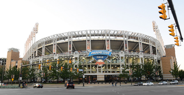
My favorite place to sit at Progressive Field is in the left-field bleachers.
From that panoramic view of home plate and both baselines, one of my more depressing between-pitch pastimes is to fixate on all of the empty seats and ponder why there aren’t people in them. I was at scores of Indians games in the late 1990s. I remember what that scene was like. What happened? Why has the market changed so drastically?
My best guess is that the answer is complicated. There would seem to be a confluence of factors to explain the precipitous drop in Indians’ attendance. I have some research in the works that will highlight one under-reported hypothesis, but that study—which will be submitted for academic publication this summer—is not complete enough for me to announce. Yet.
In the meantime, I wanted to share some of my other research on attendance at Indians games. In particular, while understanding the recent year-over-year decline in attendance involves a number of complexities, an examination of the reasons for game-to-game fluctuations in attendance within a given season is a much more straight-forward research project and offers some revealing insights about the behavior of Cleveland fans. In other words, this research article asks the following question:
How is attendance at Cleveland Indians games affected by game-specific factors?
By using readily available data from Retrosheet.org and a censored-normal regression model as applied in multiple academic papers, this research article will separate out the factors that explain attendance in a given season, including gameday opponent, day and month of the game, Indians’ win-loss record, characteristics of the starting pitchers, and a number of other variables. The results will therefore offer perspective on the ticket-buying behavior of Indians fans.
To examine this question with sufficient depth, this article will represent Part I of a multi-part series. First, I will outline the methodology and examine the determinants of Indians attendance between 2002 and 2016. To provide context, I will then compare the Indians’ results with the other four teams in the American League Central. Future articles will examine (a) how these game characteristics affect attendance for teams outside of the AL Central and (b) how these variables influenced attendance at Cleveland Stadium in its last 25 seasons (1969-1993) as the Indians’ home stadium.
(Note: If pressed for time—or patience—I have included a bullet-point list of conclusions near the bottom of the study. No one will notice if you skip ahead.)
METHODOLOGY
The study of game-by-game attendance patterns in Major League Baseball is a straight-forward process given the availability of game logs at Retrosheet. For each MLB season, Retrosheet has created a spreadsheet that has an entry for every game that year with information detailing its date, teams, location, starting lineups, attendance, etc. By combining these spreadsheets across years and writing some code to generate each team’s record and place in the standings on gameday (among other variables), I have produced a single data set that contains information on every MLB game from 1969 to 2016. After excluding a handful of games for unique circumstances—such as the Indians’ three-game “home” series in Milwaukee in 2007 and a number of games played overseas—the dataset features 104,857 observations.
An examination of attendance patterns for the Cleveland Indians reflects three distinct eras of game attendance since 1969. As demonstrated in Table 1 (below), the Indians’ dominance at the box office between 1994 and 2001 represents a historical break from attendance figures before and after that period. Average game attendance in that eight-year period (41,584) was nearly triple that of the previous 25 years (14,078) and is almost twice as much as the last 15 years (22,614). Further, the Indians had a “sellout” in 557 of 607 games during those eight seasons; in contrast, they sold out just 62 regular-season games in the last 15 years.1
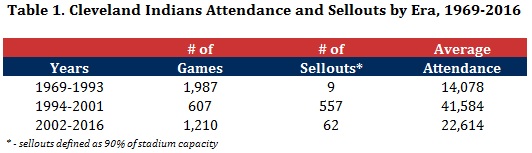
The number of sellouts is important when it comes to engaging in an analysis of the determinants of game-to-game fluctuations in attendance at Cleveland Indians games. The method that is uniformly used to evaluate the determinants of sports attendance—multiple regression—analyzes variations in the dependent variable (attendance) and attempts to attribute these fluctuations to changes in the independent variables (e.g., day of the week, gameday opponent). However, if every game is a sellout—as it was during the 455-game sellout streak—then there are no meaningful fluctuations in game-to-game attendance within a given season. In this situation, it therefore becomes impossible to evaluate the change in consumer demand for game tickets based on game characteristics given that the dependent variable is capped and doesn’t change from game to game.2
This article resolves the sellout problem—for now—by solely focusing on the third era of Indians attendance between 2002 and 2016. Before outlining the empirical guts of the article—the specification of the regression model—it is important to provide some context to the analysis by offering a basic overview of Indians attendance over this 15-year period. To lead off, Table 2 (below) reflects the average annual attendance at Indians games for each year between 2002 and 2016. As has been discussed at great lengths in Northeast Ohio, average attendance has fallen precipitously this decade; it has only once exceeded 20,000 since 2010. Consumer demand for tickets during the Indians’ playoff runs of 2013 and 2016 was particularly disappointing as the average attendance was nearly 10,000 less per game than during the Tribe’s regular-season march to the playoffs in 2007.

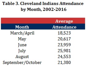
The brutal and steep decline in Indians attendance this decade is obviously worrisome, however it is reminded that the reasons for this year-over-year erosion in support rest outside the scope of this article. Instead, this study attempts to understand game-to-game attendance patterns within each season. To those ends, Table 3 (below) provides the average attendance for regular-season Indians games by each month between 2002 and 2016. The results are predictable, with attendance at its lowest in March and April, eventually peaking in July and August, and suffering a modest decline in September and October.
Examining attendance by the day of the week, Table 4 (below) also outlines a predictable pattern. Attendance is lowest on weekdays and higher on the weekends. It is notable, however, that the attendance boost on Sundays is considerable weaker than on Fridays and Saturdays.

Table 5 (below) summarizes how the Indians’ American League opponents influence gameday attendance in Cleveland. Predictably, attendance is highest when the New York Yankees come to down; average attendance against New York (31,295) substantially surpasses any other AL team. Attendance also seems to rise when Tampa Bay, Detroit and Baltimore visit Progressive Field. While Houston brings up the rear, it should be noted that a disproportionate number of Indians-Astros games have occurred after Houston switched to the AL in 2012; as noted above, Indians attendance post-2012 has been exceedingly low.

While the table above summarizes attendance by current AL opponents, Table 6 (below) provides a similar analysis for National League visitors. As somewhat expected, attendance figures for these interleague games are considerably higher. Attendance for Indians games against the Cincinnati Reds—Cleveland’s primary interleague opponent—exceeds that of all but one AL opponent. While average attendance for games against the Braves, Pirates and Diamondbacks also exceed 30,000, those teams have only made a limited number of appearances in Cleveland since 2002.

While the results of the last two tables indicate that attendance increases when the Tigers come to town—and sinks when it’s the Royals—it is important to ask whether these differences are meaningful. Perhaps MLB schedule-makers disproportionately schedule Indians-Tigers games on weekends in July. Perhaps Indians-Royals games are always during weekdays in April. If this is the case, then at least part of the attendance differentials between opponents may have nothing to do with the opponents themselves. As a result, it is imperative that any empirical analysis of attendance attempt to untangle the potentially conflating effects of gameday opponent, month of the year, day of the week, and other possible factors that affect how many people pour through the turnstiles at Progressive Field.
The need to untangle competing effects from multiple variables onto a specific outcome is a common issue in economics. As a result, the primary tool in an economist’s toolbox—multiple regression—has been applied in nearly every empirical analysis of sports attendance in the academic literature. As stated above, regression analyses examine how fluctuations in a dependent variable (in this case, attendance) can be explained by patterns among the independent variables (e.g., day of the week, gameday opponent). It is estimated as an equation, with the coefficients calculated as to minimize the sum of squared residuals between the estimated outcome and actual outcome for all observations in the sample. For more background on regression, I’d start here.
The regression model applied in this study is derived from a review of “best practices” among published academic work on MLB gameday attendance. The model employed in this article is as follows:
ln(attendance) = f(home team performance, month, day of the week, opponent characteristics, game characteristics, starting pitcher characteristics, home team year)
The inclusion of most of these variables should be straight forward. First, it is expected that individual game attendance will be heavily dependent on the performance of the home team to that point in the season; winning teams are simply expected to draw more fans. Second, month and day of the week are included to control for what is expected to be higher attendance in summer months and on weekends. Third, “opponent characteristics” is included as a series of variables that controls for the visiting team (e.g., Yankees, Orioles) as well as that team’s recent level of success. The vector of “game characteristics” includes two variables to control for the home opener and doubleheaders. As demonstrated in an article in the Journal of Sports Economics, the characteristics of a game’s starting pitcher can have significant effects on gameday attendance; as a result, both starters’ wins above replacement (WAR) and star power are included as empirically outlined in that article.
The final variable—“home team year”—is critical. If one is analyzing a sample of games that includes multiple teams and/or multiple seasons, then attendance might be higher or lower due to factors that do not fluctuate from game to game. For example, if one compared two equivalent home games in 2016—one at Fenway Park and one at Progressive Field—it would be expected that attendance would be higher in Boston for game invariant reasons. Maybe Boston’s economy is in better shape. Maybe Fenway Park is a better attraction. Maybe public transportation in Boston is more convenient. Maybe the Red Sox’s fan base is just different. Whatever the reason, a regression model that analyzes a sample featuring multiple teams and/or multiple seasons would need a way to control for those game invariant factors that cause attendance to be higher or lower in a specific location or in a specific year.3
To control for these game invariant factors, this model follows best practices in the academic literature in using a “fixed effects” approach. This means that the model includes an indicator variable—which takes on a value of 0 or 1—to control for each home team’s season included in the model. As an example, for all 81 home games hosted by the Indians in 2008, a specific variable is created that assigns those games a “1” and all other games a “0.” By including a similar variable for all team-seasons in the model, one can separate out the expected year-to-year and team-to-team differences in attendance from the fluctuations in attendance attributable to individual game characteristics.
Before describing the results of the regression analysis, it should be noted that the “sellouts” issue has not completely dissipated. While examining Indians’ attendance between 2002 and 2016 eliminates the problem of having an entire season of sellouts, there were still 62 occasions over a 15-year period where Progressive Field is effectively viewed as “sold out” as defined in this study.4 When a sellout occurs, this has the effect of “right censoring” attendance; in other words, there may be game-specific factors (e.g., Opening Day) that drives demand for tickets sky-high, but the maximum observable number of tickets sold is limited by the stadium’s capacity. Since censoring has an empirical impact on the estimated effects of the independent variables (e.g., it would decrease the estimated attendance effect of Opening Day), economists in this situation rely on censored-normal regression techniques to estimate more “true” estimates of coefficients. This method, as often applied in the academic literature on baseball attendance, is similarly employed here.5
RESULTS
Cleveland Indians Attendance
Analyzing Cleveland Indians gameday attendance between 2002 and 2016, the results from the regression model are presented in Table 7 (below). An initial diagnostic check of the results is reassuring, as the coefficients have the expected sign and their magnitudes are generally consistent with the broader research on MLB attendance.
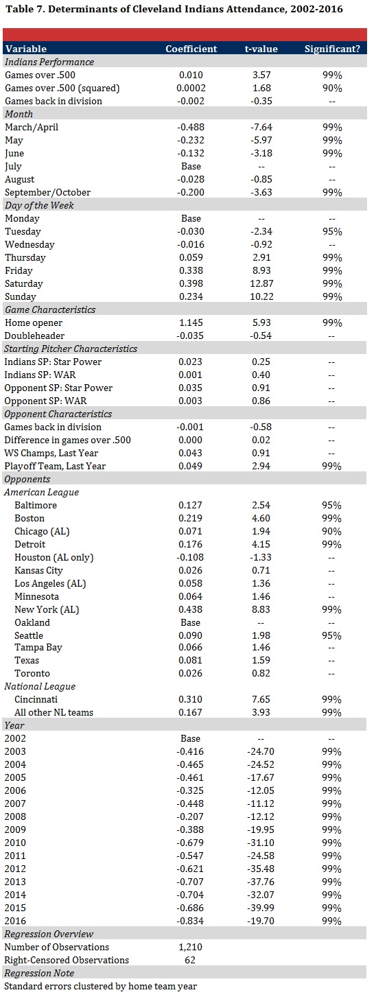
Since some portions of those reading this article may be unfamiliar with interpreting regression output, the first part of this section will be to slowly walk through each result and explain its meaning. The first variable controls for the Indians’ record as of the start of each game; the number of games above (positive) or below (negative) .500 is used in place of winning percentage given that the latter may overstate the performance of a team early in the season (i.e., a 3-0 team has a 1.000 winning percentage). The estimated coefficient on that variable—0.010—implies that as the difference between the Indians’ wins and losses (or “net wins”) improves by one, gameday attendance is expected to climb by 1.0% holding all else equal. All coefficients are similarly expressed in percentage terms given that the dependent variable has been transformed by a natural log (i.e., “ln”).
The coefficient represents one-half of the analysis on each variable. In any regression model, coefficients will be calculated for any included variable even if that factor is completely unrelated to the outcome. The issue for economists and researchers, then, is trying to separate out the important and meaningful factors from those that are simply noise. To do this, economists rely on evaluations of a coefficient’s statistical significance. This approach essentially asks whether one can be, say, 95% confident that an estimated coefficient reflects an actual—or nonzero—relationship between an independent variable (e.g., winning) and a dependent variable (e.g., attendance). If a statistical relationship fails to meet one of economists’ three typical thresholds—90%, 95% and 99% confidence—then the variable in question is typically dismissed as noise.
Returning to the first coefficient linking Indians’ record and game attendance, the results in Table 7 reflect that one can say with greater than 99% confidence that winning has a nonzero effect on gameday attendance. This, of course, is as expected. The magnitude of the coefficient indicates that the every one-game increase in net wins yields the Indians a 1.0% gain in gameday attendance in a given season. However, it would seem to be logical that a gain in net wins would more greatly impact attendance if the Indians were contending than if they were floundering; in other words, it can be hypothesized that an extra win is more important for a winning team than a losing team when it comes to attendance. To test this potential “non-linear” relationship between wins and attendance, the model includes the squared term for net wins. If net wins are more important for winning teams, then one would expect to see a quadratic relationship between the two variables (e.g., think the right-hand side of an upward-opening parabola).
The results offer some evidence to suggest that this hypothesis to be correct in Cleveland, as the coefficient on the squared term for net wins is positive and statistically significant with 90% confidence. In other words, an increase in net wins indeed impacts attendance much more when the Indians are already fielding a winning team than when compared to a more mediocre record.
But does the Indians’ relative position in the standings matter after controlling for their record? The results in Table 7 suggest that it does not. The results offer a predictably negative coefficient—indicating that more games back is correlated with lower attendance—but the t-statistic is so minute that this variable fails to be statistically significant at any reasonable threshold; in other words, it can be interpreted as noise. This is not terribly surprising; if the Indians are playing sufficiently under .500 in August, does it matter whether they are 10 games back or 20 games back? The results suggest that it does not.
Turning to the attendance effect of month, this variable is structured by including six indicator (or 0/1) variables to represent each month(s). In situations where there are a series of indicator variables, regression analyses require that one of those variables be omitted to serve as the “base” category; all the other variables are then compared to the base. In this analysis, July represents the base category. The results, therefore, demonstrate that regular-season games in March and April, holding all else equal, have 48.8% lower attendance than July games; this effect is statistically significant with 99% confidence.
The other months also demonstrate a predictable pattern. Holding all else equal, Indians home games in May (-23.2%) and June (-13.2%) also feature substantially lower attendance than July games; both effects are statistically significant with 99% confidence. In contrast, there is no discernible difference between attendance in July and August; while the coefficient indicates a slight decline in the latter month, this effect is not large enough to be deemed as statistically significant. Finally, holding all else equal, September games draw 20% fewer fans than otherwise equivalent July games, an effect that is statistically significant with 99% confidence.
An analysis of days of the week uses a similar series of indicator variables; this time, Monday games are identified as the base category. The results demonstrate that, over the course of the week, attendance at Indians game is lowest on Tuesdays; the results indicate that Tuesday games draw 3.0% fewer fans than equivalent games on Mondays, an effect that is statistically significant with 95% confidence. While Monday and Wednesday attendance is statistically indistinguishable, attendance starts to increase on Thursdays—a 5.9% increase over Mondays—before predictably exploding on the weekend.
In terms of game characteristics, the results indicate that the Indians’ home opener is expected to see an attendance boost of 114.5%, an effect that is statistically significant with greater than 99% confidence. This is expected, and the magnitude is reassuring since this would typically indicate that attendance would more than double its norm for Opening Day which, compared to season averages, would predict that Progressive Field was more or less sold out (which is true). Finally, the results indicate that doubleheaders do not affect gameday attendance at Indians games (i.e., the effect is small and not statistically significant).
The characteristics of each team’s starting pitchers do not seem to have much of an effect on gameday attendance at Progressive Field: neither the star power nor wins above replacement of either starter—both for the Indians and their opponent—have any statistically significant impact on attendance. This is not terribly surprising. As described in the aforementioned article in the Journal of Sports Economics, the relationship between starting pitcher characteristics and game attendance has been substantially weakening over the last few decades. While the JSE study did find statistically significant effects of star power on attendance across all of baseball between 1994 and 2010, the sample used was sufficiently larger—it included all 30 MLB teams—such that it was much more likely to uncover statistically significant patterns; sample size is a critical determinant of significance. It is reassuring that all of the signs of the coefficients are predictably positive—which is consistent with the earlier study—but none of the variables individually demonstrate any significant impact on Indians attendance since 2002.
Turning to the attendance impact of Indians’ gameday opponents, it does not appear as if the visiting team’s place in the standings in the current season has any effect; the coefficient on the games back variable is not statistically significant at any reasonable threshold. Further, the difference in net wins between the Indians and their opponent—a measure of “competitive uncertainty”—reflects a lack of any attendance impact. While an opponent’s current success seems to have little effect on attendance at Progressive Field, it does appear as if past success does have some influence. Holding all else equal, playoff teams from the prior year are expected to increase Indians attendance by 4.9%, an effect that is statistically significant with greater than 99% confidence. The results suggest that visiting teams who won the prior year’s World Series added an additional 4.3% increase in attendance—on top of their playoff premium—however that value fails to be statistically significant.
More important than an opponent’s success, however, appears to simply be the name on the front of their jerseys: the Indians’ gameday opponent appears to have enormous influence on attendance at Progressive Field. Using the Oakland A’s—a longstanding and seemingly “neutral” club that is not within close geographical proximity—as the base category, the results demonstrate that attendance patterns at Progressive Field fluctuate sharply based on the opponent, holding all else equal. The New York Yankees draw the biggest crowds among Cleveland’s opponents; compared to an equivalent Indians-A’s game, an Indians-Yankees contest is expected to feature 43.8% higher attendance. That is an enormous effect and is statistically significant with 99% confidence.
Other American League clubs also yield positive, albeit smaller, attendance effects that are also statistically significant. After the Yankees, the Boston Red Sox offer the next-highest attendance gains, with 21.9% more fans coming to the stadium to see Boston than they would to see an equivalent game against Oakland. Given the geographical proximity, it should not be surprising that the Detroit Tigers are next, boosting attendance by 17.6% when compared to Oakland. Other American League teams that boost attendance when compared to the A’s include Baltimore (12.7%), Seattle (9.0%) and Chicago (7.1%). While the inclusion of Seattle on this list was initially surprising, it is suspected that much of this may be attributable to the presence of Ichiro Suzuki being on the Mariners’ roster through 2012.
Turning to the analysis of National League clubs, the results clearly demonstrate that interleague play matters to Cleveland fans. A lot. The results indicate that attendance at an Indians-Reds game is expected to be 31.0% higher than an equivalent Indians-A’s game. Condensing all other NL teams into a single variable (since the Indians only infrequently play specific NL clubs, as evident in Table 6), the results demonstrate that any non-Cincinnati National League team is also expected to increase attendance in Cleveland by 16.7% over and above an equivalent game against Oakland. Both effects are statistically significant with 99% confidence.5

The bottom section of Table 7 outlines the year-to-year fluctuations in Indians attendance attributable to game invariant factors. With 2002 serving as the base year, the negative and statistically significant coefficients in all subsequent years reflect the substantial decline in Indians attendance in the 15 years after the expiration of the sellout streak. The numbers also predictably indicate the steep drop off in attendance in 2010 as the Indians were in the midst of the second straight 90-loss season, a decline in attendance to which the franchise has never seemingly recovered. It is especially noteworthy that the largest negative coefficient was estimated for 2016. While the average attendance figures for last season (19,650) were not the team’s worst since the Progressive Field in the 15 years of the sample, the largest negative coefficient (-0.834) for 2016 indicates that attendance last season was the worst it has been at Progressive Field after controlling for game-variant characteristics (e.g., their AL Central-winning 94-67 record).6
American League Central Attendance
While the results described above detail the ticket-buying behavior of Cleveland Indians fans, are these responses to changes in game characteristics similar to those of fans of other clubs? Yes, Indians fans make ticket-purchasing decisions based on the day of the week, gameday opponent, and other game-variant components. But how does this compare to the hometown fans of, say, the rest of the American League Central? Are Cleveland fans unusual in any way in comparison to their Midwestern counterparts?
In terms of game-to-game characteristics, the results of the model for other AL Central clubs indicate that Cleveland fans’ ticket-purchasing behavior is largely similar to other fan bases in the division. To demonstrate this, Table 8 (below) presents the results of the attendance model for all five teams in the AL Central. For the sake of space and simplicity, the table only reflects the coefficient for each team; the coefficient is presented in red if it is statistically significant with at least 95% confidence.

In terms of home team performance, the first section of Table 8 reflects that fans of all five teams seem to react similarly to an increase in their team’s net win total. While the shape (linear vs. quadratic) of the relationship between wins and attendance is slightly different across each of the five clubs, the magnitude and general direction is largely the same: in general, every one-unit increase in net wins is more or less associated with a 1% increase in attendance.
Turning to month of the year, the results reflect how geography and weather impact seasonal baseball attendance. While attendance for all five teams follows a parabolic curve that peaks in the summer months, the timing and size of that peak differs across the division. It is likely not coincidence that attendance in Chicago, Cleveland and Detroit follow a near-identical path. In these outdoor stadiums on the Great Lakes, attendance suffers mightily in March and April before slowly warming up with the weather to peak in July and August; it then suffers a substantial decline in September as the weather cools back down.
In contrast, the month-to-month fluctuations in Kansas City are far less extreme. This is predictable given the more temperate springs in western Missouri and eastern Kansas, as April attendance for the Royals is relatively closer to their July attendance. Compared to the rest of the division, Kansas City uniquely experiences (a) a significant decline in attendance in August vis-à-vis July and (b) a much smaller attendance decline in September. While attendance for the Minnesota Twins also reflect a unique pattern—including a clear and significant peak in August instead of July—a month-by-month analysis is complicated by the fact that the Twins played in the climate-controlled Metrodome through 2009.
In terms of days of the week, every team in the AL Central predictably demonstrates higher attendance on the weekend, with crowds peaking on Saturday. But beyond that, the results offer some intriguing differences between the fan bases of AL Central clubs. First, it would appear as if attendance at White Sox games is unusually high on Mondays; it is 12%-16% higher than the next three days of the week and statistically indistinguishable from Fridays. In contrast, the Twins experience their worst gameday attendance on Mondays, with every other day reflecting a positive and statistically significant relationship when compared to the first day of the workweek. Second, while Thursdays offer a significant attendance boost in Cleveland, Detroit and Minnesota, it seems to have no effect in Chicago or Kansas City.
An overview of the next four sections of Table 8 reflects some small, but unique, characteristics in attendance patterns in the AL Central. For example, fans in Detroit and Minnesota demonstrate a statistically significant responsiveness to a game’s starting pitchers that is not evident elsewhere. Investigating this more deeply, however, much of this effect is attributable to former Cy Young-winners Justin Verlander (Detroit) and Johan Santana (Minnesota).7 This is finding is consistent with the Journal of Sports Economics article that demonstrated that any attendance effects of starting pitchers since 1994 is largely isolated to the very few superstar pitchers in baseball at the time.
In terms of opponent characteristics, it does appear that the opponent has a stronger effect in some cities than others. For example, while last season’s playoff teams offer a statistically significant boost in attendance in Cleveland and Minnesota, these clubs have a negligible effect elsewhere in the division. Further, while the prior year’s World Series champion increases attendance by 10.0% when visiting the White Sox in Chicago, the estimated effect is much smaller and fails to be statistically significant for the other four teams in the AL Central.
Turning to individual opponents, the results of Table 8 demonstrate that the decision to purchase tickets by all five fan bases is considerably influenced by the home team’s game day opponent. As compared to each team’s respective base opponent—chosen as the long-standing American League team with the worst visiting attendance—some consistent and predictable patterns emerge. First, visits by the Yankees and Red Sox increase attendance for all five AL Central teams; these effects are strongest in Cleveland and Kansas City. Second, the geographical proximity of a visiting team’s fan base matters. Attendance increases at both stadiums whenever Cleveland plays Detroit or when Chicago plays Minnesota; further, the influx of Canadian fans seemingly fuels a significant increase in attendance at Twins games whenever they host the Blue Jays.
From the results of Table 8, it also appears that interleague play matters for every team in the division. Some of the largest attendance premiums are attached to each club’s most frequent interleague rival since 2002. Predictably, these effects are strongest for the White Sox (a 69.3% attendance increase vs. the Cubs when compared to an equivalent game against the A’s) and the Royals (a 55.9% increase vs. the Cardinals when compared to the Angels), however they are also large and significant for the other three clubs in the division. Further, interleague games against other National League teams increases attendance between 10% to 20% when compared to each respective team’s base opponent in the model.8
Finally, the bottom portion of Table 8 provides the effects of year-to-year attendance changes attributable to game-invariant effects. At first glance, the results demonstrate a clear difference in Cleveland; while the Indians have seen their attendance fundamentals decline sharply since 2002, all four other clubs have had near uniform increases since that time. While initially alarming from a Cleveland standpoint, the results actually make sense from a historical perspective. Looking back at attendance in 2002, the Indians were coming down from the glory years of the late 1990s while all four other clubs were struggling at the box office: the Tigers and White Sox failed to average 20,000 per game, while the Royals and Twins barely squeaked above that line. While attendance increased slightly in the subsequent years for all four teams, it then skyrocketed for each of the teams following a World Series appearance (Chicago, 2005; Detroit, 2006; Kansas City, 2014) or the opening of a new stadium (Minnesota, 2010). Unfortunately, it is too soon to say definitively how the Indians’ appearance in the 2016 World Series will change the franchise’s attendance patterns, but evidence within the division suggests that it could have considerable effects.
Conclusions & Caveats
This study analyzed how the characteristics of each game affected individual game attendance in Cleveland and the rest of the American League Central between 2002 and 2016. A quick summary of the findings suggest:
- A one-game increase in “net wins” (wins minus losses) is associated with an approximately 1.0% improvement in game attendance at Progressive Field, with an effect that increases modestly as the Indians’ record improves. This effect is largely consistent with the relationship between winning and attendance as estimated for the other four teams in the AL Central.
- Attendance at Indians games predictably peaks in July and experiences considerable sluggishness in colder weather months; the attendance pattern in Cleveland is nearly identical to other AL Central teams with outdoor stadiums on the coast of the Great Lakes (Chicago, Detroit). Attendance weakness in the early spring and late summer is far less of a concern in the warmer climate of Kansas City, where attendance peaks a bit earlier in the year.
- Cleveland attendance demonstrates a predictable pattern by day of the week, bottoming out on Tuesdays before climbing significantly on Thursdays leading into enormous attendance increases on the weekend. While this pattern is largely consistent with the other four teams in the division, some idiosyncrasies are visible in the data (e.g., Monday attendance is exceedingly high in Chicago and unusually low in Minnesota).
- Indians fans do not seem to react to the star power or recent performance of a game’s starting pitchers. This is not unique among fans in the AL Central, although the fan bases in Detroit (Justin Verlander) and Minnesota (Johan Santana) have demonstrated significant increases in attendance when certain pitchers are starting.
- Cleveland attendance is considerably influenced by the gameday opponent. First, attendance increases by 4.9% whenever the Indians host a playoff team from the prior year; this effect far exceeds that of the rest of the division. Second, individual opponents have enormous effects on attendance. While this is true for all five AL Central teams, the effects seem slightly more pronounced in Cleveland. For the Indians, the largest attendance effects are attributable to visits by the Yankees and Reds, with each boosting attendance by more than 30% compared to the base category; the Red Sox, Tigers and Orioles also produce double-digit percentage increases.9 Looking across all five teams in the division, it is clear that (a) interleague play has significant attendance affects and (b) geographical proximity of an opponent’s fan base is a critical factor in predicting a potential attendance effect.
- While not the central focus of this study, the results do reflect the 15-year decline in attendance at Progressive Field. After controlling for the Indians’ 94-67 record and other game characteristics in 2016, the results reflect that attendance last season was the worst that it has been since the stadium opened. Every other AL Central team has seen their attendance clearly move in the opposite direction since 2002, however (a) all four of those teams were struggling for attendance in 2002 (unlike Cleveland) and (b) the attendance patterns for each club substantially improved only after a World Series trip (Chicago, Detroit, Kansas City) or the opening of a new stadium (Minnesota).
The results of this study may not have offered any eye-opening revelations; it should be common sense that gameday attendance at Progressive Field is impacted by team performance, opponent and day of the week. However, this analysis was designed to provide perspective on the relative magnitudes of each effect. How much does the Indians’ win-loss record matter? How much does the opponent matter? How much does attendance increase on a Friday?
This study not only attempted to answer those questions, but also provided a series of comparisons by presenting the results for the same model estimated for the other four teams in the American League Central. The results indicate that the game-to-game ticket-buying behavior of Cleveland fans is largely consistent with the fan bases across the rest of the division, even if some idiosyncrasies exist.
While hopefully this analysis of game-to-game patterns in Indians attendance was insightful, it is recognized that none of this was designed to answer the most important attendance question in Cleveland: why has it declined so sharply on a year-to-year basis since 2002? As alluded to in the introduction, this question is complicated and likely represents a confluence of factors. I suspect that this will be a regular topic on this blog in the future, but it is not something directly addressed in this study.
Before concluding, it is important to acknowledge the shortcomings of this study. Every microeconomics paper ever written can seemingly be critiqued for omitting critical variables; this study is no different. In particular, there are three variables that are noticeably absent in the model: weather, dynamic pricing, and promotions. The exclusion of these variables does not invalidate the model, but their exclusion does create the potential for “omitted variable bias” that one must consider when evaluating the estimated effects of other variables.
Among these three omitted variables, weather conditions are indirectly controlled for by the inclusion of the month variables in the model; the incorporation of weather conditions into the model would have allowed this study to separate out the effects of temperature and precipitation from other month-related effects (e.g., school being in session). Dynamic pricing and promotions in Major League Baseball are two variables that have been the subject of some academic review (see here and here), however the data collection requirements for these variables to cover all MLB games between 2002 and 2016 range from incredibly difficult (promotions) to impossible (dynamic pricing).10 It is likely that the exclusion of these variables are picked up elsewhere in the model—such as the attendance boost attributable to the Indians’ fireworks shows appearing in the large Friday coefficient—but it would not be expected that the omission of these variables would fundamentally alter the relationships expressed in the results.
Finally, note that regression estimates are calculated as the average effects for each team over a 15-year period. However, it should therefore be reminded that some of the coefficients presented in this study have been trending up or down during this time and may not be predictive of future trends. As an example, it is quite possible that the significant attendance premium in Cleveland attributable to games against the Mariners was a largely a byproduct of Ichiro Suzuki’s time on Seattle’s roster through 2012. If that is the case, then it would be unwise to project that Indians-Mariners games will continue to exhibit higher attendance vis-a-vis other opponents in 2016 and beyond.
Footnotes
1: One of the more irritating issues in working with MLB attendance data is that there is no known database that identifies a game to be a “sellout.” However, even with known sellouts—such as the Indians’ 455-game streak from 1995 to 2001—the listed attendance is typically less than that of stadium capacity. As a result, I have subsequently defined a sellout to be games where attendance is more than 90% of stadium capacity. While this approach will undoubtedly mislabel a small number of games as sellouts, higher thresholds fail to recognize known sellouts. While imperfect, the 90% threshold has been an accepted empirical approach that I have used in my published academic work.
2: Analyzing consumer demand in a season full of sellouts would be possible if one had data on ticket prices for sold out games on the secondary market (e.g., StubHub); higher ticket prices would reflect higher demand. But I am not aware of this data existing in the public sphere and I doubt it even exists anywhere for Indians games between 1994 and 2001.
3: Traditionally, the use of fixed effects techniques to control for game invariant characteristics would include a team’s ticket pricing. However, the increased use of dynamic pricing models that change ticket prices based on opponent, month or day of the game would necessarily undermine this assumption. That said, I am unaware of any data on teams’ dynamic pricing strategies that are available in the public sphere; as a result, it is not yet something that can be incorporated into a non-proprietary attendance model.
4: As explained in footnote one, a reminder that a “sellout” is defined as whenever attendance is 90% of stadium capacity.
5: The results in Table 7 should be construed as the average interleague effect between 2002 and 2016. It cannot be ruled out that the premium attached to interleague play has declined over time.
6: An alternative specification of the regression model was estimated using 2016 as the base year category. All other years were deemed to have a positive and statistically significant coefficient—with 99% confidence—against 2016.
7: Since Verlander joined the Tigers in 2005, the average home attendance in his starts (excluding home openers) has been 34,519; when any other pitcher has started since that time, average attendance has fallen to 33,555. The effect is much larger in Minnesota when Johan Santana started. Between 2002 and 2007—Santana’s last year with the Twins—the average home attendance in his starts (excluding home openers) was 27,241; in contrast, average attendance fell to just 24,806 in games started by other Twins pitchers during that time period.
8: As pointed out in Footnote 5, it is important to again consider that the interleague results in Table 8 should be interpreted as the average interleague effect between 2002 and 2016; it is possible that this effect has eroded over time.
9: While not included in the results, a separate model was estimated that pulled out Indians-Pirates games from all other interleague games hosted in Cleveland; the results indicated that the Pirates also increased attendance at Progressive Field by greater than 30% compared to an equivalent game against the base category (Oakland). While this effect was statistically significant, it was not presented in the results given that Pittsburgh has only visited Cleveland for nine total games since 2002.
10: Given that the Indians—and all other MLB teams—likely have internal data on their dynamic pricing model, it is likely that the front office has compiled proprietary studies understanding its effect on attendance. That said, this information is not available in the public sphere.
